5. Appendix
In this section we provide a summary about the task of each file in the toolbox in Table (Table 5.1).
Function |
Task |
|---|---|
\(\texttt{error\_number=Check\_inputs}\) \(\texttt{(hObject,type,varargin)}\) |
Check inputs of parameters to determine possible errors in the neural dynamic simulation part. |
\(\texttt{validation=Check\_inputs\_NPD(handles)}\) |
Check inputs of parameters to determine possible errors in neural populations (de)synchronization part. |
\(\texttt{runable=check\_port\_eval(handles)}\) |
Activate/deactivate check boxes according to the number of selected options in the neural dynamic simulation part. |
\(\texttt{check\_port\_show(handles,flag)}\) |
Make checkboxes visible/invisible according to the selected models in the neural dynamic simulation part. |
\(\texttt{u=control\_input(handles,domain,}\) \(\texttt{Z,Zp,L2,omega,i,dt,varargin)}\) |
Specify the value of control input according to the control strategy in neural populations (de)synchronization part. |
\(\texttt{control\_user\_defined\_choise(handles)}\) |
If there exists the user-defined control input file, open it; otherwise, create a new Matlab file. |
\(\texttt{[phi,L2,thetas,u,sim\_time,x]=}\) \(\texttt{decoupled\_FD(handles,M,flag)}\) |
Apply the finite difference method to solve the population-level partial differential equation of uncoupled neural oscillators. |
\(\texttt{[rho,V,thetas,U,sim\_time,domain]=}\) \(\texttt{decoupled\_Fourier(handles,M,flag)}\) |
Apply the Fourier decomposition method to solve population-level partial differential equation of uncoupled neural oscillators. |
\(\texttt{[phi,L2,thetas,u,sim\_time,domain]=}\) \(\texttt{decoupled\_RBF(handles,M,flag)}\) |
Applying the radial basis function method to solve the population-level partial differential equation of uncoupled neural oscillators. |
\(\texttt{[phi,L2,thetas,u,sim\_time,domain]=}\) \(\texttt{decoupled\_RBFFD(handles,M,flag)}\) |
Apply the radial basis function generated finite difference method to solve the population-level partial differential equation of uncoupled neural oscillators. |
\(\texttt{[phi,L2,thetas,u,sim\_time,domain]=}\) \(\texttt{decoupled\_spectral(handles,M,flag)}\) |
Apply the spectral method to solve the population-level partial differential equation of uncoupled neural oscillators. |
\(\texttt{[dist,diff\_dist]=dist\_def(dist\_model,}\) \(\texttt{location,concentration,omega,i,}\) \(\texttt{dt,domain)}\) |
Specify the initial and final distributions in neural populations (de)synchronization part. |
Function |
Task |
|---|---|
\(\texttt{[DM] = DistanceMatrix(ds,cnt,differ)}\) |
Construct the distance matrix of radial basis function.` |
\(\texttt{valid=error\_handling(handles,type)}\) |
Handle the possible errors and extensions. |
\(\texttt{par=getparams(handles)}\) |
Set the values of parameters in the neural dynamic simulation part. |
\(\texttt{temp4=init\_tetha(population,}\) \(\texttt{phi,N,domain)}\) |
Set the initial phases of neural oscillators in the neural populations (de)synchronization part. |
\(\texttt{Initialize\_Dynamic(handles,varargin)}\) |
Initialize the parameter of the HH dynamical system by loading the neural dynamic simulation part for the first time. |
\(\texttt{varargout = NeuronDynamic(varargin)}\) |
Load the neural dynamic simulation window. |
\(\texttt{u=noisy\_control\_input(handles,domain,}\) \(\texttt{Z,Zp,L2,B,omega,i,dt,varargin)}\) |
Specify the value of noisy system control input according to the control strategy in neural populations (de)synchronization part. |
\(\texttt{[phi,L2,thetas,u,sim\_time,x]=}\) \(\texttt{noisy\_decoupled\_FD}\) \(\texttt{(handles,M,flag)}\) |
Apply the finite difference method to solve the noisy population-level partial differential equation of uncoupled neural oscillators. |
\(\texttt{[rho,V,thetas,U,sim\_time,domain]=}\) \(\texttt{noisy\_decoupled\_Fourier}\) \(\texttt{(handles,M,flag)}\) |
Apply the Fourier decomposition method to solve the noisy population-level partial differential equation of uncoupled neural oscillators. |
\(\texttt{[phi,L2,thetas,u,sim\_time,domain]=}\) \(\texttt{noisy\_decoupled\_RBF}\) \(\texttt{(handles,M,flag)}\) |
Applying the radial basis function method to solve the noisy population-level partial differential equation of uncoupled neural oscillators. |
\(\texttt{[phi,L2,thetas,u,sim\_time,domain]=}\) \(\texttt{noisy\_decoupled\_RBFFD}\) \(\texttt{(handles,M,flag)}\) |
Apply the radial basis function generated finite difference method to solve the noisy population-level partial differential equation of uncoupled neural oscillators. |
\(\texttt{[phi,L2,thetas,u,sim\_time,domain]=}\) \(\texttt{noisy\_decoupled\_spectral}\) \(\texttt{(handles,M,flag)}\) |
Apply the spectral method to solve the noisy population-level partial differential equation of uncoupled neural oscillators. |
\(\texttt{varargout = NPDlab(varargin)}\) |
The first function which runs by starting the toolbox. |
\(\texttt{OK\_Panel(handles)}\) |
Set upper and lower bounds in the neural dynamic simulation part. |
\(\texttt{OptionPanelActive(handles,flag)}\) |
Make slide bar and checkboxes enable or disable according to the models the neural dynamic simulation. |
\(\texttt{Output\_plots(handles,peak,durT,x,phi}\) \(\texttt{,phif,sim\_time,u,L2,cos\_thetas,}\) \(\texttt{sin\_th)}\) |
Display the results of the control model in the figures in the neural dynamic simulation part. |
\(\texttt{pause\_popup\_change(handles)}\) |
Do proper actions when the pause button is pressed in neural populations (de)synchronization part. |
\(\texttt{[STEPS,result]=PlotsDynamic(handles)}\) |
Display the selected variables figures. |
\(\texttt{Popup\_changes\_init(handles)}\) |
Prepare the options of the neural dynamic simulation panel according to the selected dynamical model. |
\(\texttt{popup\_Distribution\_change}\) \(\texttt{(H,handles,type)}\) |
Prepare the option of initial or final distributions according to the selected distribution in neural populations (de)synchronization part. |
\(\texttt{popup\_PRC\_change(H,handles)}\) |
Consider a default value for the period according to the selected model in neural populations (de)synchronization part. |
Function |
Task |
|---|---|
\(\texttt{Portrait(handles,H,vector,}\) \(\texttt{ flag,varargin)}\) |
Display the phase portrait, stream, and vector field figure in the neural dynamic simulation part. |
\(\texttt{PortraitDynamic(handles)}\) |
Send the parameters to \(\texttt{Portrait}\) function. |
\(\texttt{[z,zp]=PRC\_function(model,}\) \(\texttt{method,domain)}\) |
Compute PRC function and its derivative according to the selected neural model in the neural populations (de)synchronization part. |
\(\texttt{[prc,dprc] = PRC\_interpol}\) \(\texttt{(domReg,type)}\) |
Interpolate HH and Thalamic neuron PRC functions and their derivatives. |
\(\texttt{Report(handles,varargin)}\) |
Report some information in the bottom panel in the neural dynamic simulation part. |
\(\texttt{report\_last(H,domain,u,L2,}\) \(\texttt{thetas,phi,iter)}\) |
Report some information in the bottom panel in the neural populations (de)synchronization part. |
\(\texttt{report\_main(handles,location,}\) \(\texttt{concentration,omega,i,dt,domain)}\) |
Recognize the type in phenomena in the neural populations (de)synchronization part. |
\(\texttt{L=RK\_stoc(tts,u,T,dt,D,prc,type)}\) |
Apply fourth-order Runge-Kutta to solve the stochastic ODE to determine the phase of the noisy oscillator in the neural populations (de)synchronization part. |
\(\texttt{L=RK4control(tts,u,T,dt,prc,type)}\) |
Apply fourth-order Runge-Kutta to solve the ODE to determine the phase of the oscillator in the neural populations (de)synchronization part. |
\(\texttt{[res,dt]=RKb(varargin)}\) |
Solving the neural dynamical systems. |
\(\texttt{[Dist,Error,Thetas,U,Sim\_time,}\) \(\texttt{Domain]=Run\_test(handles,flag)}\) |
Run the designed test case in the neural populations (de)synchronization part. |
\(\texttt{show\_error(error\_number)}\) |
Show the related error message when an error occurs in the toolbox. |
\(\texttt{Start\_Action(handles)}\) |
Make enable or disable the objects in the window when the simulation is started/paused/stopped in the neural populations (de)synchronization part. |
\(\texttt{start\_model(handles)}\) |
Call required functions when the start button is pressed to start the simulation in the neural populations (de)synchronization part. |
\(\texttt{stream(H,func,y1val,y2val,}\) \(\texttt{t,varargin)}\) |
Draw the 2D stream of dynamical systems in the neural dynamic simulation part. |
\(\texttt{stream3d(H,func,y1val,y2val,}\) \(\texttt{t,varargin)}\) |
Draw the 3D stream of dynamical systems in the neural dynamic simulation part. |
\(\texttt{u=user\_defined\_control(varargin)}\) |
The user can define his own control strategy in this function. |
\(\texttt{[dist,diff\_dist]=}\) \(\texttt{user\_defined\_final\_dist(domain,}\) \(\texttt{omega,i,dt)}\) |
The user can define a new final distribution in this function. |
\(\texttt{[dist,diff\_dist]=}\) \(\texttt{user\_defined\_initial\_dist}\) \(\texttt{(domain,omega,i,dt)}\) |
The user can define a new initial distribution in this function. |
\(\texttt{vectfield(H,func,y1val,y2val,}\) \(\texttt{t,varargin)}\) |
Draw 2D vector field of dynamical systems in the neural dynamic simulation part. |
\(\texttt{vectfield3d(H,func,y1val,y2val,}\) \(\texttt{t,varargin)}\) |
Draw 3D vector field of dynamical systems in the neural dynamic simulation part. |
\(\texttt{[X,DX,DY,DDX,DDY,DXY] =}\) \(\texttt{ Wendland(eps,differ,type,r,x,y)}\) |
Define Wendland functions and their derivatives. |
As you can see, NPDS Toolbox contains more than 50 functions. We provide a diagram (See Figure Arch) to display the architecture of the toolbox functions and relations between them. In this figure, the sources of graphical user interface files are represented by rectangles. We have two main part i.e \(\texttt{NPDSLab.m}\) and \(\texttt{NeuronDynamic.m}\). These files are the main parts of the toolbox, which are represented by two diamonds and can be run from the command line directly. Moreover, \(\texttt{About.m}\) can be run from the command line, but it is not one of the main files of the toolbox and just gives a brief overview of the toolbox. This file is shown by a diamond in the figure. There are some main functions. These functions call the other functions to do their task correctly. On the other hand, regular functions are called by the main ones and these functions do not need to call other functions. These two types of functions are displayed by two ellipses and one ellipse, respectively. Some functions invoke simple functions defined inside the same file. Simple functions are shown by the ellipse dotted line. A diamond inside a rectangle expresses a static file that creates a user-defined function file when the user intends to define a new function. Finally, the cloud-like shape is \(\texttt{PARAMETER\_GUIDE.md}\) file which is a guide for model parameters.
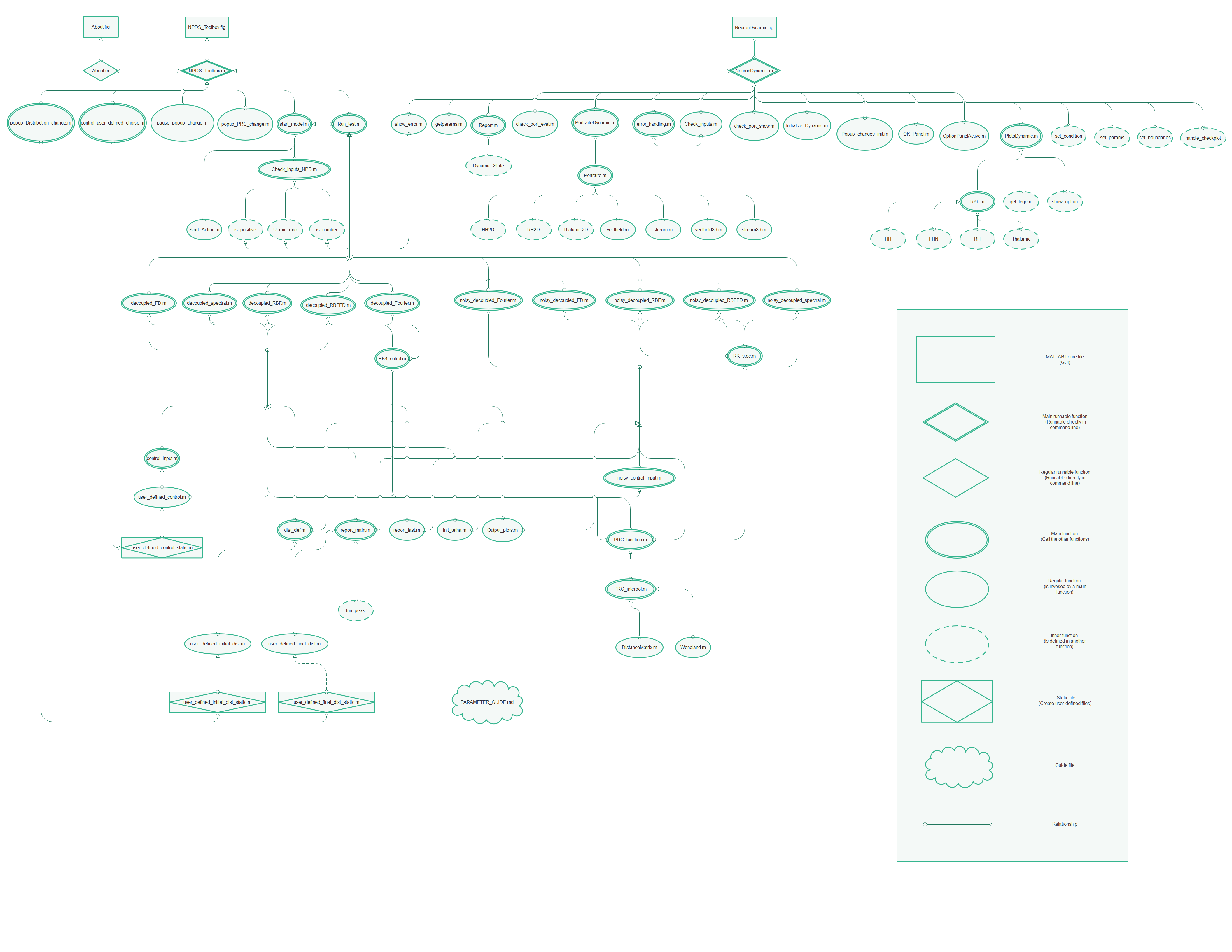
Fig. 5.1 The architecture of NPDS Toolbox (Click on the image to see it in the actual size)